FADGI in Practice
Refining Toward Better Performance
As we learned the practical implications of measurements such as Delta-e values and Nyquist Frequency, we expanded our technical vocabulary. We sought out resources to learn our new jargon like ImageZebra’s guide. We learned how to interpret the data and it became easier to iterate our physical setups to produce higher measuring results until we were able to meet our goals efficiently.
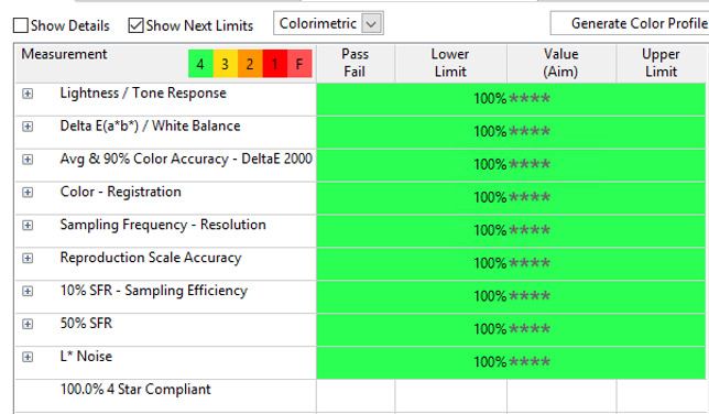
What do we do when our testing results don't look, excitingly, like these 100% 4-star measuring shown above?
Here are some of the ways we've learned to interpret the data and respond to it:
Lightness / Tone Response
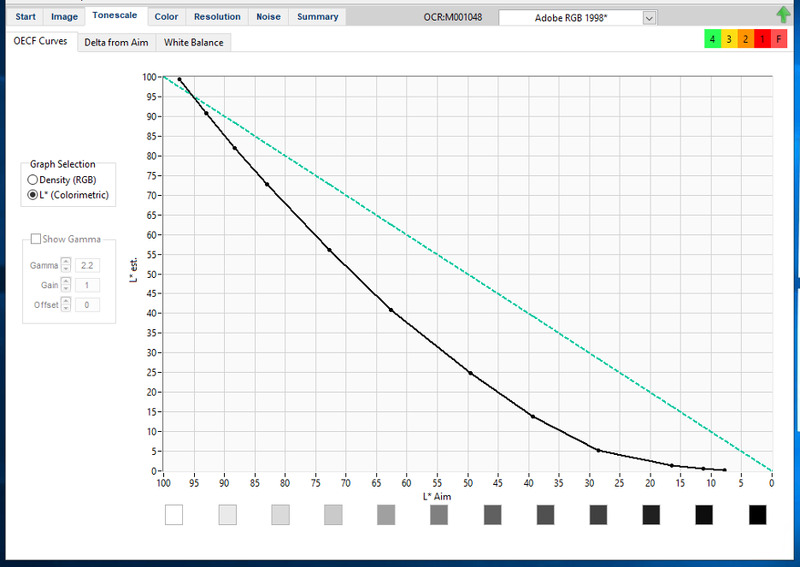
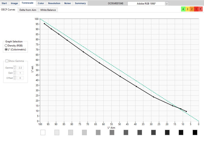
- This is addressed via exposure -- our existing practices aligned closely with the target measurements for this metric. In order to decrease the distance in the measured and captured tonescale values in our photography setups, we have introduced s-curve adjustments in the luma channel and custom ICC profiles (custom color profile) when needed. We nearly always proceed with the latter solution since it has yielded more accurate results on our systems. Maintaining a consistent capture environment by eliminating reflections and light pollution is important for this metric as well. We have gray walls, blocked ceiling lights that are turned off, blackout shades, and gray or black lab coats when needed to help maintain a consistent and not-full-of-odd-reflections environment. We rarely use flatbed scanners in our workflow, but we are just now embarking on incorporating FADGI into baseline measurements for them in alignment with our other stations. Below is an example of how the visualized data from the target file images can help explain an image quality issue that is easy to see once you have something consistent to compare on the equipment (in this case, we tested a collaborating unit's flatbed scanner they use for reproductions for reference purposes to help resolve the issue of scans that appeared overly dark).
Delta E(a*b*) / White Balance
- We white balance on the 13 patch of our item level targets, as much of our materials are lighter, this lighter gray value works well for us. We use linear scientific curves almost exclusively, resulting in a flat aesthetic with a lot of information. We rarely use linear responsive curves and when we do, it's for items that are highly reflective or there is clipping data (blown out) in the highlights. If any of this is off, this metric might show issues.
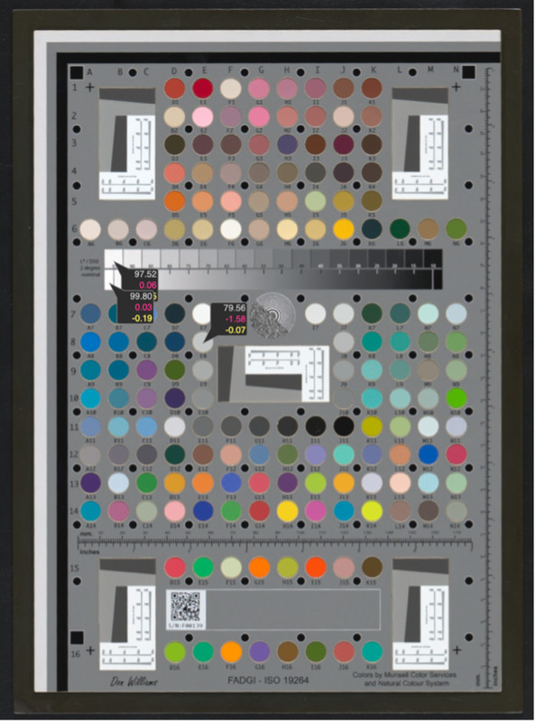
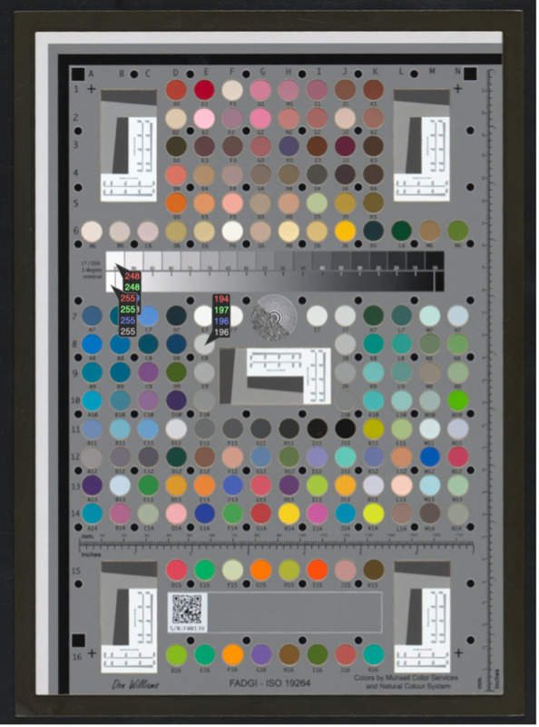
Screenshot of exposures for our FADGI - ISO 19264 target with color readout values in LAB and sRGB colorspaces for a file used to create a custom ICC profile. We've found this file needs to be slightly brighter, by up to 8 points in sRGB, than our aim for validation targets or daily calibration targets. We use this dedicated FADGI device level target to create custom ICC profiles and validate, or check our performance with a different object level target.
Avg & 90% Color Accuracy - DeltaE 2000
- This measures the difference between the measured colors on the targets we utilize and the measured L*ab values on the digitized image. Ideally, values reported in our image evaluation software should result in a low DeltaE 2000 value of less than 3 -- if when evaluated this value is above our accepted tolerance, we create a custom ICC profile for that scene or apply a more appropriate ICC profile. Additionally, we ensure that our white balance and exposures are accurate throughout the image. As long as the tonescale metrics measure favorably, our cameras and lights can easily achieve this DeltaE 2000 metric consistently throughout capture sessions. Ensuring accurate focus, dusting/cleaning, and photographing at 1/125s shutter speed also helps minimize any ambient light interference with color reproduction.
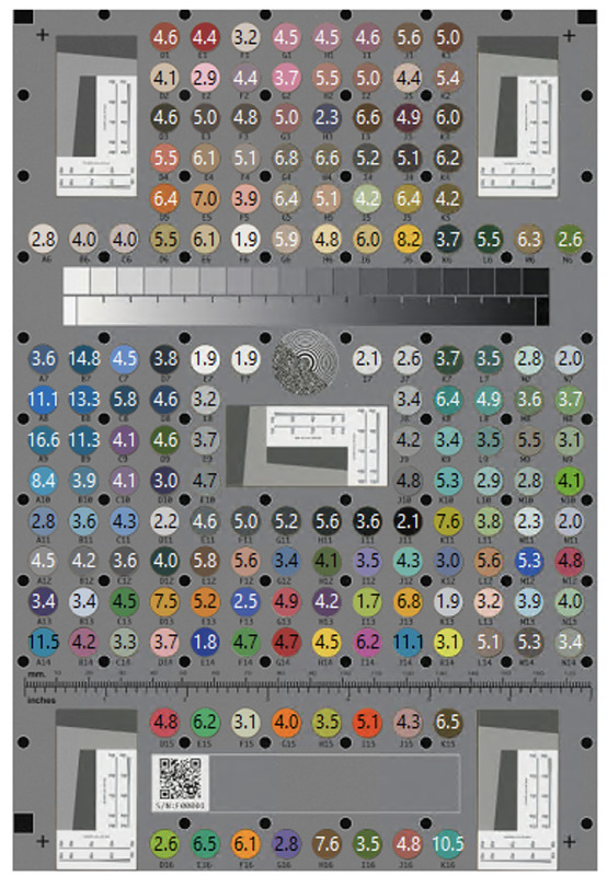
Delta E Value Measurements from a Flatbed Scanner illustrated here show some blue/teal areas suffered, as they measure higher than 10. Overall this target evaluates mostly Fadgi 3 star for color accuracy, which is good for most uses.
Color - Registration
- This is rarely an issue and often resolves once other metrics are improved. The varying color channels will show different results as the software reads the horizontal and vertical regions of interest (ROIs). These also measure SFR (more on that later), so if these ROIs aren't aligned well in the initial test, that can also throw the measurements off. We do use Lens Cast Calibrations (LCCs) which are like flat fielding masks in other workflows – these tweak the files to even the lighting through processing steps in the software. LCCs (white or gray boards) need to be shot at the same aperture as the setup, and without any clipped (overly bright) areas. Careful LCC creation is important for these to function accurately and not negatively affect color (we adjust lights or shutter speed to darken the image around 1 stop to achieve intended exposure for these).
Sampling Frequency - Resolution
- This specifically refers to the pixels per inch (ppi) the image was captured at (concerning the distance of the camera to the item in relation to the lens focal length and camera's sensor size), not what the file derivate was output as. For example, a 1 for 1 print of a 600ppi reproduction could be printed at 600dpi (dots per inch) and be accurately sized to the original. That same item could be digitized at a different resolution, either farther away or closer to the item, and output as a 600ppi file, but when that file is printed at 600dpi, it will be bigger or smaller than the original, depending on if the camera was closer or farther from the item, and will not be a 1 for 1 scale reproduction without resampling the file. You can resize a file's ppi to meet any number of uses, but the specific resolution in this metric is measured optically by the software looking at the dark gray dots on the targets being measured and calculating what ppi, in terms of distance to the item, the target was photographed at.
Reproduction Scale Accuracy
- This evaluation metric ties in closely with sampling frequency by comparing the output resolution (ppi) to the captured resolution (metric above). For example, a photograph would need to be captured at a minimum of 600ppi to be considered a FADGI 4-star image for this evaluation parameter. The amount in which the captured (spatial) ppi deviates from the exported ppi has an accepted tolerance of + or - 6 pixels per inch for a FADGI 4-star image. The closer the captured ppi is to the target ppi, the higher the potential star rating would be for this metric. One can adjust any image file's ppi at any point in the workflow, but after the image is captured, it merely changes the density of pixels and does not increase the resolved detail in the image.
10% SFR - Sampling Efficiency
- This looks at the gray slant line areas of the tested targets. This Spatial Frequency Resolution has been improved for us by refining focus on the surface of the object, leveling the plane of the target to the plane of the camera sensor (we use a laser to do this), and shooting within the sharpest aperture for our camera systems. We've found f/6.3 creates the sharpest image, as compared to the smaller f/9 aperture which is prone to softness due to image diffraction. When using autofocus, the location of the target in the capture frame can also affect this metric -- focusing near a corner of a frame helps ensure tack sharp focus throughout our image edge to edge.
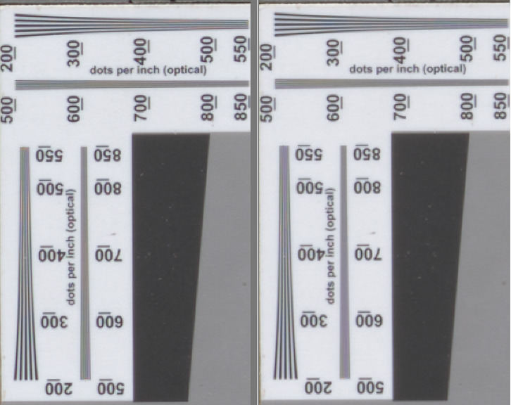
Screenshot Detail Comparing Optical Image Resolution: the left side converging lines are visible farther into the 600ppi regions than the right side.
50% SFR (Spatial Frequency Response)
- Is what we’re capturing optically as high a resolution as we think it is (in the graph below, reaching near the Nyquist Frequency)? This metric looks at the gray slant line areas of the tested targets. It has been a bit more challenging to rectify when measurements indicated something is off with this metric since it can be affected by a variety of in-camera and environmental factors. If this metric is performing poorly when analyzed, we first check the camera planarity with our laser level to ensure the camera and capture plane are perfectly aligned. Applying minimal sharpening in the post-processing phase is a tool we've tried and ultimately have not adopted to fix this metric. We add custom minimal sharpening to our access derivative files and remove all sharpening from our preservation file derivative TIFs. Artificial sharpening improves this metric, but we found through practice when all other metrics measure well this SFR does too, rendering the sharpening unnecessary. Added contrast helps: lens flare was shared with us as a culprit to poor SFR results from collaboration with other institutions, so we’ve also mitigated this with block card flags outside our lenses on our dual capture system. They function like extra big lens hoods, giving us a little boost in image quality. Limiting vibrations is helpful too, which could look as simple as slowing the pace of digitization down slightly, so movement doesn't negatively affect the images.
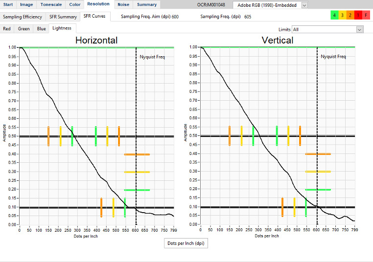
Spatial Frequency Response (SFR) Curve Graphs, the results here of a happy target image illustrated by the smooth data line reaching FADGI 4-star image goal posts.
Noise
- When shooting at a higher ISO setting, such as we do at our dual capture system, our noise settings in software are minimally applied to all files. For other stations we can turn the noise adjustments off, as this has not been a metric we have had issues with. Given the high image quality our specialized camera equipment produces, noise is generally not a concern.
Testing Schedule
We now aim to measure at 80% or higher 4-Star Compliant at our stations. We test at the beginning of each project block (which can vary from weekly to each semester depending on the schedule and priorities). Our goal in testing is to ensure consistency, provide high quality imaging that's measurable, and monitor our equipment for potential maintenance needs.
The testing workflow looks something like this:
- Shoot object level target & output at preservation file specifications
- Move object level target file to server
- Download object level target from server onto remote Windows virtual machine
- Run object level target through software
- Interpret analyzed results of object level target and adjust workspace as needed
- Retest as needed
Possible additional ICC profiling steps if that adjustment is needed:
- Shoot FADGI device level target
- Move object level target file to server
- Download object level target from server onto remote Windows virtual machine
- Run object level target through software and generate ICC profile
- Move ICC profile into ColorSynch folder on workstation
- Restart Imaging software and apply new ICC profile to repeat testing steps above with an object level target
We shoot daily targets for every session and item level targets for each item we digitize. We have an internal practice of comparing our daily target's visually for focus, color and exposure to a "Best Bet Target" (one that tested well at the beginning of our setups that measured 80% compliant or better in our FADGI testing). Through this practice, we can have daily assurances we are accurate in our settings and setups, without slowing down daily to test and iterate, and each project we can work to improve our FADGI ratings and image quality. This close attention to detail has led us to finding a sharper aperture to shoot at, leading to better focus and more consistent evaluations of our equipment and performance.
Previous Section:
FADGI Process
Next Section: